stream - Streamlines of plotfile vector

Given a plotfile containing a vector field and an MEF file containing a collection of “seed” points, create “streamlines” eminating from the seed points that are locally parallel to the vector field. The resulting streamlines will be of a fixed length going both directions along the vector field from the seed point. Results will be written in a custom plotfile-like data folder, which is discussed in the data section. These files cannot be directly visualized with standard plotfile tools.

Usage:
   ./stream2d.gnu.MPI.ex plotfile=<string> [options]
     Options:
         isoFile=<string>  OR  seedLoc=<real real [real]
         streamFile=<string>  OR  outFile=<string>
         is_per=<int int int> (DEF=1 1 1)
         finestLevel=<int> (DEF=finest level in plotfile)
         progressName=<string> (DEF=temp)
         traceAlongV=<bool> (DEF=0)
         buildAltSurf=<bool> (DEF=0)
             (if true, requires altVal=<real>, also takes dt=<real> (DEF=0) and altIsoFile=<string>)
         nRKsteps=<int> (DEF=51)
         hRK=<real> (DEF=.1 (*dx_finest in plotfile)
         nGrow=<int> (DEF=4)
         bounds=<float * 4> (DEF=NULL)

Options

Seed points

Streamlines are computed to emanate from seed points specified by the user. The seed points can be defined as the nodes of a triangulated surface (in 3D) or a “polyline” (2D), or can be specified directly in the ParmParsed input.

If a triangulated surface or polyline is used (by passing the name of the MEF file via the isoFile keyword), the resulting streamlines retain the connectivity inferred by the input structure. And since the steamlines will not, in general, cross they will bound a triangular-prism shaped volume extending a distance from the surface on either side. The union of these volumes tile a layer around the original triagulated surface. In 2D, the streamlines will bound a polygonal structure that similarly tiles the region around the original polyline.

If the seed points are specified directly in the input, no connectivity information is inferred. Currently, the only option for this mode is accessible via the seedLoc keyword, which specifies the coordinates of a single seed point.

Integration options

Figure 4 illustrates a streamline (in black) that is computed from a vector field, whose components are specified on cell centers. The paths are integrated in both directions from the seed point, as depicted in 4. The user specifies the interval, \(h\), as a fraction, hRK, of the grid spacing at the finest level of vector field used, as well as the total number of such intervals, nRK.

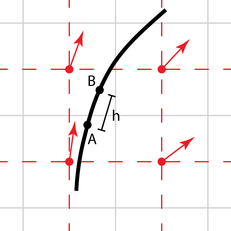
4 Streamlines (in black) are computed by integrating the vector field from a seed point in intervals of \(h\), e.g., from point A to B, using the RK4 scheme. The vector field components are defined at the nodes of the dual grid connecting the cell centers and are linearly interpolated.

Vector field

Currently, the vector field can be constructed to align with the gradient of a scalar field, or with the flow velocity (if the option traceAlongV = t). If the the velocity field is not used, the required components of the gradient vector field (identified via the keyword, progressName) are computed on the fly with second-order centered differences.

Alt surface

If the keyword buildAltSurf = t, a new triangulated surface is constructed after the streamlines are generated. This surface will be created where the scalar identified as progressName takes the value specified by the keyword, altVal along the streamlines. The connectivity of this surface will be identical to the connectivity of the original surface (specified with the keyword, isoFile). The new surface is written to the file indicated by the keyword, altIsoFile.

Algorithm details

The algorithm starts by determining the finest AMR level box in the plotfile (indicated by the keyword, plotfile) that contains the physical location of each seed point (up to and including the level indicated by the keyword, finestLevel). Then, as the required plotfile data is read (in parallel), a distribution map will be created for each level, and we use this to assign the processor that will be responsible for computing the streamline associated with that point.

The RK4 scheme is used to integrate the vector field, \(u\), along streamline for a distance \(h\) from A to B (see Figure 4):

\[\begin{split}x_{B} =& \;x_{n} + \frac{1}{6} \big( k_1 + 2 k_2 + 2 k_3 + k_4\big)\\ &k_1 = h \, u(x_{A}), \;\; x_{1} = x_{A} + 0.5 k_{1}\\ &k_2 = h \,u(x_{1}), \;\; x_{2} = x_{A} + 0.5 k_{2}\\ &k_3 = h \,u(x_{2}), \;\; x_{3} = x_{A} + k_{3}\\ &k_4 = h \,u(x_{3})\end{split}\]

The vector field \(u\) is defined at cell-centers and we need to construct a function that, given the vector field data at nodes, is able to linearly interpolate these components as needed to evaluate the above expressions. A simple way to orchestrate this interpolater is to base it on source data that lives on a logically rectangular, uniformly space grid, as this allows simple/fast “mod” operations to locate the specific source data indices for the interpolation.

However, if the seed point starts off, for example, near the boundary of the owning box, it is possible that the integration will eventually step off the grid, and possibly across AMR levels, before reaching the required path length, and thus attempt to access data that is unavailable to this processor. A simple solution follows the usual AMReX approach in these situations - grow cells. Given the hRK and nRK parameters, we can compute the size of a grow region buffer that is guaranteed to fully contain the path - even if it is rather large - see Figure 5. And given the standard AMReX fill-patching infrastructure, we can fill the required data locally from the plotfile classes, being careful to account for periodic and physical domain boundaries.

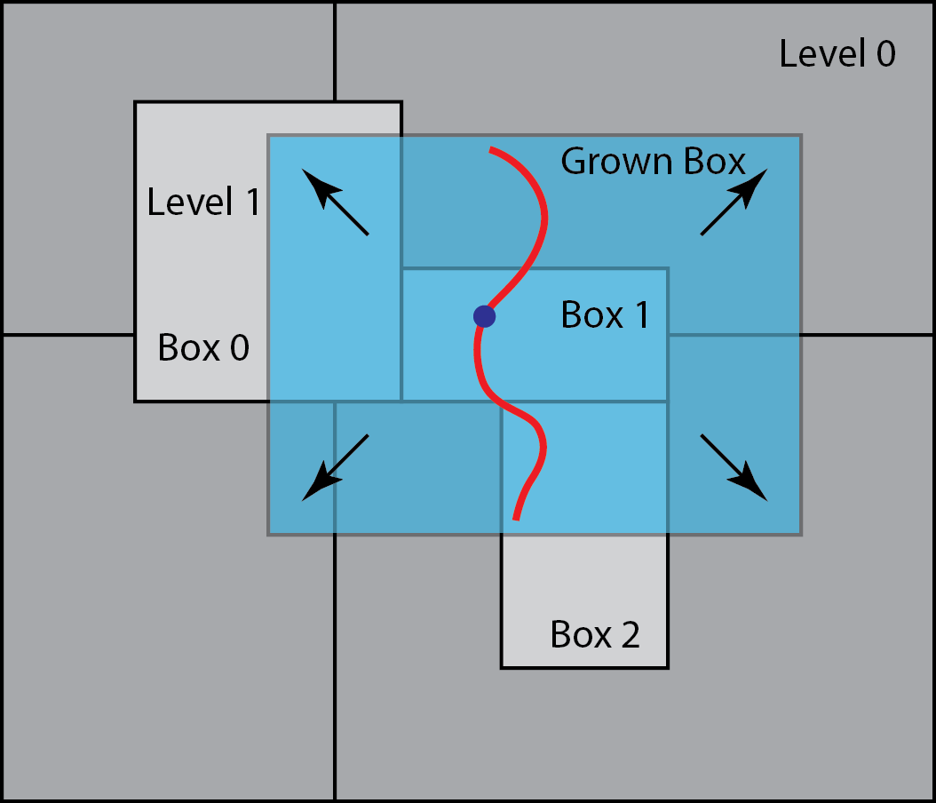
5 A streamline (red) is generated from the seed point (blue), which is owned by Box 1 in the finest level here, Level 1. The streamline goes beyond the valid region of Box 1. Data to fill the grown box is copied from neighboring grids at the same refinement level, and interpolated from coarse levels where needed.

Note that because the size of the grow region needed depends on the maximum length of the streamlines, these patches can be quite large, particularly in 3D. However, this approach is far simpler than any method that might move between levels and/or processors whenever boundaries are crossed. In order to manage very large datasets, this tool has been written to run in parallel with MPI. For maximum flexibility, there is also a separate tool that can read the streamline generated with the above strategy, and interpolate a set of fields onto the streamlines.